Next: Line Width - Size Up: Introduction Previous: Density Distribution Contents
We have seen that a molecular cloud consists in many molecular cloud cores. For many years, there are attempts to determine the mass spectrum of the cores.
From a radio molecular line survey, a mass of each cloud core is determined.
Plotting a histogram of number of cores against the mass,
we have found that a mass spectrum can be fitted by a power law as
| (1.18) |
| Paper | Region | Observation | Mass range | |
| Loren (1989) |
|
|||
| Stutzki & Guesten (1990) | M17 SW | C |
|
|
| Lada et al. (1991) | L1630 | CS ( |
|
|
| Nozawa et al. (1991) |
|
|||
| Tatematsu et al. (1993) | Orion A | CS ( |
|
|
| Dobashi et al. (1996) | Cygnus |
|
||
| Onish et al (1996) | Taurus | C |
|
|
| Motte, André, & Neri (1998) |
|
|||
|
|
||||
| Testi & Sargent (1998) | Sarpens |
|
||
| Kramer et al.(1998) | L1457 etc |
|
||
| Heithausen et al. (1998) | MCLD 123.5 + 24.9, Polaris Flare |
|
||
| Johnstone et al. (2000) |
|
|
||
|
|
||||
| Johnstone et al. (2001) | Ori B |
|
|
|
| Onishi et al. (2002) | Taurus | H |
|
|
| Ikeda, Sunada, & Kitamura (2007) | Ori A | H |
|
|
|
|
||||
| Ikeda & Kitamura (2009) | Ori A | C |
|
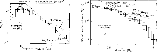 |
Figure 1.31(left) (André, Ward-Thomson, & Barsony 2000)
shows a mass spectrum function ![]() for 59
for 59
![]() Oph cloud prestellar cores obtained
at the IRAM 30-m telescope with the MPIfR 19-channel bolometer array.
Presetellar cores with a mass
Oph cloud prestellar cores obtained
at the IRAM 30-m telescope with the MPIfR 19-channel bolometer array.
Presetellar cores with a mass ![]() has a spectrum of
has a spectrum of
![]() (
(![]() ) for
) for
![]() .
While the right panel (Motte et al 2001) shows the cumulative mass spectrum
(
.
While the right panel (Motte et al 2001) shows the cumulative mass spectrum
(![]() vs.
vs. ![]() ) of the 70 starless condensations identified in NGC 2068/2071.
The mass spectrum for the 30 condensations of the NGC 2068 sub-region is very similar in shape.
The best-fit power-law is
) of the 70 starless condensations identified in NGC 2068/2071.
The mass spectrum for the 30 condensations of the NGC 2068 sub-region is very similar in shape.
The best-fit power-law is
![]() above
above
![]() .
That is,
.
That is, ![]() .
This power derived from the dust thermal emission is different from that derived by the radio
molecular emission lines.
Table 1.1 summarizes the observations to calculate
the power index of core mass function.
.
This power derived from the dust thermal emission is different from that derived by the radio
molecular emission lines.
Table 1.1 summarizes the observations to calculate
the power index of core mass function.
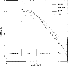
The mass fuction of newborn stars is called as initial mass fuction (IMF).
IMF for field stars in the solar neighborhood has been obtained
as shown in Figure 1.33.
The most famous one is Salpeter's IMF as
![]() (Salpeter 1955).
The low-mass end is flatter than that of
(Salpeter 1955).
The low-mass end is flatter than that of
![]() as
as
![]() for
for
![]() while
while
![]() for
for
![]() (Meyer et al. 2000).
The powers of stellar (
(Meyer et al. 2000).
The powers of stellar (
![]() )
and prestellar (
)
and prestellar (![]() ) mass functions are similar.
If one prestellar core forms one star, the stellar mass
) mass functions are similar.
If one prestellar core forms one star, the stellar mass ![]() is
proportional to the prestellar core mass as
is
proportional to the prestellar core mass as
![]() and
and
![]() , the mass spectrum of prestellar cores
completely determines the IMF.
, the mass spectrum of prestellar cores
completely determines the IMF.
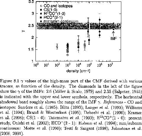
Figure 1.32 plots the power-law indices
against the typical gas densities of respective observations,
in which the critical density is taken as a typical density for
molecular line studies.
The power-law index is an increasing function
of the typical gas densitiy ![]() (Ikeda 2007) and
the cores with
(Ikeda 2007) and
the cores with
![]() have
the same power-law index as the IMF.
This may indicates these cores are the sites of star formation or
direct parents of new-born stars1.1.
have
the same power-law index as the IMF.
This may indicates these cores are the sites of star formation or
direct parents of new-born stars1.1.
 |
Kohji Tomisaka 2009-12-10