Next: Virial Analysis Up: Super- and Subsonic Flow Previous: Steady State Flow under Contents
Stellar winds are observed around various type of stars. Early type (massive) stars have large luminosities; the photon absorbed by the bound-bound transition transfers its outward momentum to the gas. This line-driven mechanism seems to work around the early type stars. On the other hand, acceleration mechanism of less massive stars are thought to be related to the coronal activity or dust driven mechanism (dusts absorb the emission and obtain outward momentum from the emission).
Here, we will see the identical mechanism in ![]() 2.8.1 and
2.8.1 and ![]() 2.8.2
works to accelerate the wind from a star.
Consider a steady state and ignore
2.8.2
works to accelerate the wind from a star.
Consider a steady state and ignore
![]() .
The continuity equation (2.1) gives
.
The continuity equation (2.1) gives
| (2.94) |
| (2.95) |
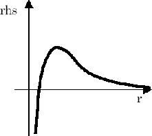
For simplicity, we assume the gas is isothermal. The rhs of equation (2.98) varies shown in Figure 2.7. Therefore, near to the star, the flow acts as the cross-section of nozzle is decreasing and far from the star it does as the cross-section is increasing. This is the same situation that the gas flows through the Laval nozzle.
Using a normalized distance
![]() ,
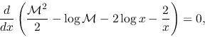
equation (2.98) becomes
,
equation (2.98) becomes
 |
(2.100) |
| (2.101) |
| (2.102) |
| (2.103) |
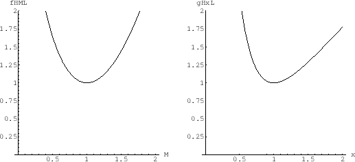
Since the minima of ![]() and
and ![]() are respectively
are respectively ![]() and
and ![]() ,
the permitted region in
,
the permitted region in ![]() changes for the values of
changes for the values of ![]() .
.
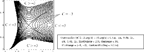 |
Out of the two solutions of ![]() , a wind solution is one with increasing
, a wind solution is one with increasing ![]() while departing from the star.
This shows us the outflow speed is slow near the star but it is accelerated and a supersonic wind blows
after passing the critical point.
Since the equations are unchanged even if we replace
while departing from the star.
This shows us the outflow speed is slow near the star but it is accelerated and a supersonic wind blows
after passing the critical point.
Since the equations are unchanged even if we replace ![]() with
with ![]() , the above solution is valid for an
accreting flow
, the above solution is valid for an
accreting flow ![]() .
Considering such a flow, the solution running from the lower-right corner to the upper-left corner represents
the accretion flow, in which the inflow velocity is accelerated reaching the star and finally accretes on the star surface
with a supersonic speed.
.
Considering such a flow, the solution running from the lower-right corner to the upper-left corner represents
the accretion flow, in which the inflow velocity is accelerated reaching the star and finally accretes on the star surface
with a supersonic speed.
Kohji Tomisaka 2012-10-03