Next: Local Star Formation Process Up: Galactic Scale Star Formation Previous: Group Velocity Contents
In the preceding section, we have seen that a spiral pattern of density perturbation is made
by the gravitational instability in the stellar system with
![]() .
This forms a grand design spiral observed in the
.
This forms a grand design spiral observed in the ![]() -band images which represent the mass distribution
which consists essentially in less-massive stars.
The amplitude of the pattern is smaller than that observed in
-band images which represent the mass distribution
which consists essentially in less-massive stars.
The amplitude of the pattern is smaller than that observed in ![]() -band images.
In this section we will see how the distribution early type stars is explained.
[Recommendation for a reference book of this section: Spitzer (1978).]
-band images.
In this section we will see how the distribution early type stars is explained.
[Recommendation for a reference book of this section: Spitzer (1978).]
Gas flowing through a spiral gravitational potential, even if its amplitude is relatively small,
acts rather nonlinearly.
Consider the gravitational potential in the sum of an axisymmetric term, ![]() and a
spiral term
and a
spiral term ![]() .
The spiral gravitational field is rotating with a pattern speed
.
The spiral gravitational field is rotating with a pattern speed
![]() .
We use a reference frame rotating with
.
We use a reference frame rotating with
![]() .
.
![]() , where
, where ![]() and
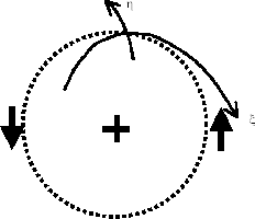
and ![]() are radial (
are radial (![]() ) and azimuthal (
) and azimuthal (![]() ) component of the flow velocity.
Consider the reference system rotating with the angular rotation speed
) component of the flow velocity.
Consider the reference system rotating with the angular rotation speed
![]() .
We assume the variables with suffix 0 represent those without the spiral potential
.
We assume the variables with suffix 0 represent those without the spiral potential ![]() and
variables with suffix 1 are used to express the difference between before and after
and
variables with suffix 1 are used to express the difference between before and after ![]() is added.
is added.
![]() ,
, ![]() , and
, and
| (3.46) | |||
| (3.47) | |||
| (3.48) | |||
| (3.49) |
| (3.56) | |||
| (3.57) | |||
| (3.58) | |||
| (3.59) |
Equations (3.53), (3.54), and (3.55) are solved under the periodic boundary condition:
![]() .
Since equation (3.54) is similar to the equations in
.
Since equation (3.54) is similar to the equations in ![]() 2.8,
you may think the solution seems like Figure 2.6.
However, it contains a term which expresses the effect of Coliois force
2.8,
you may think the solution seems like Figure 2.6.
However, it contains a term which expresses the effect of Coliois force
![]() ,
the flow becomes much complicated.
,
the flow becomes much complicated.
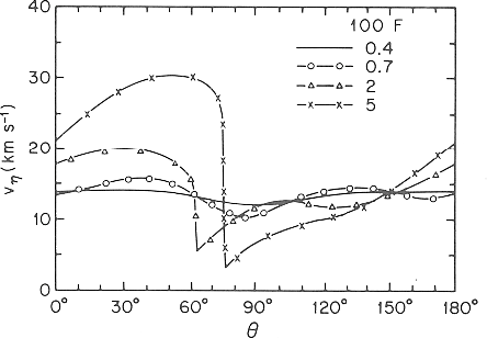
Taking care of the point that a shock front exists for a range of parameters, the solution of the above equations
are shown in Figure 3.13.
Numerical hydrodynamical calculations which solve equations (3.50), (3.51), and (3.52) was done and steady state solutions are obtained (Woodward 1975).
It is shown that ![]() %, the velocity (
%, the velocity (![]() : velocity perpendicular to the wave) does not show
any discontinuity.
In contrast, for
: velocity perpendicular to the wave) does not show
any discontinuity.
In contrast, for ![]() %, a shock wave appears.
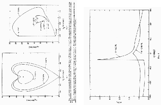
Steady state solution is obtained from the ordinary differential equations (3.53)
(3.54), and (3.55) by Shu, Milione, & Roberts (1973).
Inside the CR,
%, a shock wave appears.
Steady state solution is obtained from the ordinary differential equations (3.53)
(3.54), and (3.55) by Shu, Milione, & Roberts (1973).
Inside the CR, ![]() (Gas has a faster rotation speed than the spiral pattern).
As long as
(Gas has a faster rotation speed than the spiral pattern).
As long as ![]() there is no shock.
Increasing the amplitude of the spiral force
there is no shock.
Increasing the amplitude of the spiral force ![]() , an amplitude of the variation in
, an amplitude of the variation in ![]() increases and finally
increases and finally
![]() becomes subsonic partially.
When the flow changes its nature from supersonic to subsonic, it is accompanied with a shock.
(An inverse process, that is, changing from subsonic to supersonic is not accompanied with a shock.)
becomes subsonic partially.
When the flow changes its nature from supersonic to subsonic, it is accompanied with a shock.
(An inverse process, that is, changing from subsonic to supersonic is not accompanied with a shock.)
In the outer galaxy (still inside CR) since
![]() decreases with the the distance from the galactic center,
decreases with the the distance from the galactic center,
![]() decreases.
In this region,
decreases.
In this region,
![]() and the flow is subsonic if there is no spiral gravitational force,
and the flow is subsonic if there is no spiral gravitational force, ![]() .
In such a circumstance, increasing
.
In such a circumstance, increasing ![]() amplifies the variation in
amplifies the variation in ![]() and
and ![]() finally reaches the sound speed.
Transonic flow shows again a shock.
finally reaches the sound speed.
Transonic flow shows again a shock.
Summary of this section is:
 |
 |
![\begin{displaymath}
v_0=R(\Omega-\Omega_{\rm P})=R\left[\left(\frac{1}{R}\frac{...
...ial \Phi_0}{\partial R}\right)^{1/2}-\Omega_{\rm P}\right],
\end{displaymath}](img945.png)