Virial Analysis
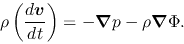
Hydrodynamic equation of motion using the Lagrangean time derivative [eq.(A.3)] is
 |
(4.17) |
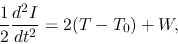
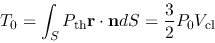
Multiplying the position vector r and integrate over a volume of a cloud, we obtain the Virial relation as
 |
(4.18) |
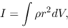
where
 |
(4.19) |
is an inertia of the cloud,
 |
(4.20) |
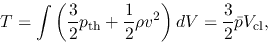
is a term corresponding to the thermal pressure plus turbulent pressure,
 |
(4.21) |
comes from a surface pressure, and
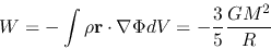 |
(4.22) |
is a gravitational energy.
To derive the last expression in each equation, we have assumed the cloud is spherical and uniform.
Here we use a standard notation as the radius  , the volume
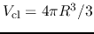 ,
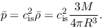
the average pressure
,
the average pressure  , and the mass
  .
.
To obtain a condition of mechanical equilibrium, we assume  .
Equation (4.18) becomes
.
Equation (4.18) becomes
 |
(4.23) |
Assuming the gas is isothermal
 , the average pressure is written as
 |
(4.24) |
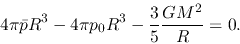
Using equation (4.24) to eliminate  from equation (4.18),
the external pressure is related to the mass and the radius as
from equation (4.18),
the external pressure is related to the mass and the radius as
 |
(4.25) |
Keeping constant and increasing from zero,  increases first, but it takes a maximum,
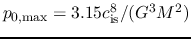 , and finally declines.
This indicates that the surface pressure must be smaller than
, and finally declines.
This indicates that the surface pressure must be smaller than
 for a cloud
to be in the equilibrium.
In other words, keeping and changing , it is shown that has a maximum value to
have a solution.
The maximum mass is equal to
for a cloud
to be in the equilibrium.
In other words, keeping and changing , it is shown that has a maximum value to
have a solution.
The maximum mass is equal to
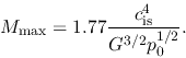 |
(4.26) |
The cloud massive than  cannot be supported against the self-gravity.
This corresponds to the Bonnor-Ebert mass [eq.(4.9)],
although the numerical factors are slightly different.
cannot be supported against the self-gravity.
This corresponds to the Bonnor-Ebert mass [eq.(4.9)],
although the numerical factors are slightly different.
Subsections
Kohji Tomisaka
2012-10-03