Dynamical Collapse
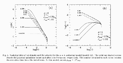
Figure 4.8:
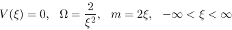
Evolution of isothermal clouds massive than the Bonnor-Ebert mass.
Density (left) and velocity (right) distributions are illustrated.
Solid lines show the cores of the preprotostellar phase (prestellar core)
and dashed lines show those of protostellar phase (protostellar core).
The evolution of the protostellar phase is studied by the sink-cell method, where
we assume the gas that entered in the sink-cells is removed from finite-difference grids
and add to the point mass sitting at the center of the sink-cells which corresponds to a protostar.
 |
In 1969, Larson (1969) and Penston (1969) found a self-similar solution which is suited for the
dynamical contraction.
Figure 4.8 is a radial density distribution for a spherical collapse of an isothermal
cloud, where the cloud has a four-times larger mass than that of the Bonnor-Ebert mass.
Although the figure is taken from a recent numerical study by Ogino et al (1999),
a similar solution was obtained in Larson (1969).
We can see that the solution has several characteristic points as follows:
- The cloud evolves in a self-similar way.
That is, the spatial distribution of the density (left) at
 is well fitted by that
at
is well fitted by that
at  after shifting
in the
after shifting
in the  and the
  directions.
As for the infall velocity spatial distribution, only a shift in the direction is needed.
directions.
As for the infall velocity spatial distribution, only a shift in the direction is needed.
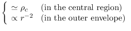
- The density distribution in the envelope, which is fitted by
 , is almost unchanged.
Only the central part of the cloud (high-density region) contracts.
, is almost unchanged.
Only the central part of the cloud (high-density region) contracts.
- The time before the core formation epoch (the core formation time
 is defined as
the time at which the central density increases greatly)
is a good indicator to know how high the central density is.
That is, reading from the figure, at
is defined as
the time at which the central density increases greatly)
is a good indicator to know how high the central density is.
That is, reading from the figure, at  () the central density reaches
 and at
  () the density is equal to
 .
This shows the maximum (central) density is approximately proportional to
.
This shows the maximum (central) density is approximately proportional to  ,
which is reasonable from the description of the free-fall time
,
which is reasonable from the description of the free-fall time
 .
.
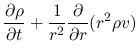
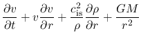
The basic equations of spherical symmetric isothermal flow are
where  represents the mass included in the radius
  and
and  denotes the mass
of the protostar.
A self-similar solution which has a form
denotes the mass
of the protostar.
A self-similar solution which has a form
 |
 |
 |
(4.66) |
 |
|
 |
(4.67) |
 |
|
 |
(4.68) |
 |
|
 |
(4.69) |
should be found, where  and
and  are functions only on
  .
For example, equation (4.66) asks the shape of the density distribution is the same
after resizing of equation (4.69)
.
For example, equation (4.66) asks the shape of the density distribution is the same
after resizing of equation (4.69)
 and re-normalizing
 as
as  .
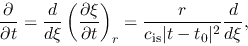
Since
.
Since
 |
(4.70) |
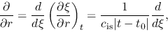
and
 |
(4.71) |
the basic equations for the spherical symmetric model yield
 |
(4.72) |
![\begin{displaymath}
\left[(\xi-V)^2-1\right]\frac{d V}{d \xi}=\left[\Omega(\xi-V)-\frac{2}{\xi}\right](\xi-V),
\end{displaymath}](img1229.png) |
(4.73) |
,
\end{displaymath}](img1230.png) |
(4.74) |
Equations (4.73) and (4.74) have a singular point at which  or
or
 .
Since the point of
.
Since the point of  const moves with
  , the flow velocity relative to this const is equal to
 .
Thus the singular point
.
Thus the singular point  at which corresponds to a sonic point.
Therefore, since the flow has to pass the sonic point smoothly,
the rhs of equations (4.73) and (4.74) have to be equal to zero at the singular point .
This gives at the sonic pont
at which corresponds to a sonic point.
Therefore, since the flow has to pass the sonic point smoothly,
the rhs of equations (4.73) and (4.74) have to be equal to zero at the singular point .
This gives at the sonic pont  ,
,
 |
(4.75) |
which leads to
 |
(4.76) |
 |
(4.77) |
These equations (4.72), (4.73) and (4.74) have an analytic solution
 |
(4.78) |
This is a solution which agrees with the Chandrasekhar's SIS.
Generally, solutions are obtained only by numerical integration.
 the solution have to converge to an asymptotic form of
This shows that for sufficiently large radius the gas flows with a constant inflow velocity
 .
.
Figure 4.9:
A self-similar solution indicating a dynamical collapse of isothermal spherical cloud (Larson-Penston solution).
Spatial distribution of the density and inflow velocity which are expected from the self-similar solution are plotted.
Dashed lines show the evolution prestellar core and solid lines show that of protostellar core.
Taken from Hanawa (1999).
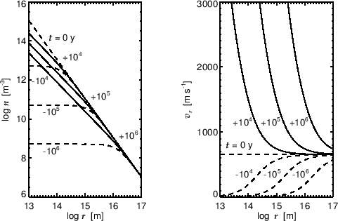 |
This has a solution in which the density and the infall velocity should be regular with
reaching the center ( ).
Such kind of solution is plotted in Figure 4.9 (left) and
Figure 4.9 (right) with
).
Such kind of solution is plotted in Figure 4.9 (left) and
Figure 4.9 (right) with  .
This time evolution is expected from the self-similar solution.
This shows that
.
This time evolution is expected from the self-similar solution.
This shows that
Reaching the outer boundary the numerical solution (Fig.4.8)
differs from the self-similar solution (Fig.4.9).
For example,  is reduced to zero in the numerical simulations, while it reaches a finite value 3.28
in the self-similar solution.
And as for the density distribution,
is reduced to zero in the numerical simulations, while it reaches a finite value 3.28
in the self-similar solution.
And as for the density distribution,  drops near the outer boundary in the numerical
simulations while it decreases proportional to
.
However, in the region except for the vicinity of the outer boundary
the self-similar solution expresses well the dynamical collapse of the spherical isothermal cloud.
This solution gives the evolution of a pre-protostellar core formed in a supercritical cloud/cloud core.
drops near the outer boundary in the numerical
simulations while it decreases proportional to
.
However, in the region except for the vicinity of the outer boundary
the self-similar solution expresses well the dynamical collapse of the spherical isothermal cloud.
This solution gives the evolution of a pre-protostellar core formed in a supercritical cloud/cloud core.
Subsections
Kohji Tomisaka
2012-10-03