Accretion Rate
Using equation (2.26), the necessary time for a mass-shell at  to reach the center
(free-fall time) is expressed as
to reach the center
(free-fall time) is expressed as
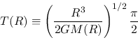 |
(4.93) |
(for detail of this section see Ogino, Tomisaka, & Nakamura 1999).
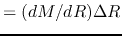
Consider two shells whose initial radii are and  .
The time difference for these two shells to reach the center
.
The time difference for these two shells to reach the center  can be written down using equation (4.93) as
![\begin{displaymath}
\Delta T(R)
=\frac{\pi{R}^{1/2}}{2^{3/2}(GM(R))^{1/2}}
\left[\frac{3}{2}-\frac{{R}}{2M(R)}\frac{dM(R)}{dR}\right]\Delta R.
\end{displaymath}](img1318.png) |
(4.94) |
Mass in the shell between and ,
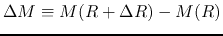
 , accretes
on the central object in .
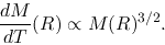
Thus, mass accretion rate for a pressure-free cloud is expressed
as
, accretes
on the central object in .
Thus, mass accretion rate for a pressure-free cloud is expressed
as
 .
This leads to the expression as
.
This leads to the expression as
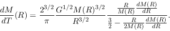 |
(4.95) |
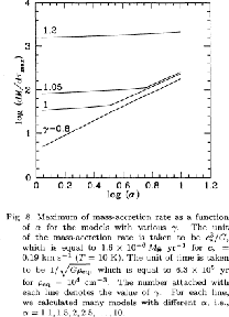
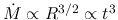
Figure 4.11:
Mass accretion rate against the typical density of the cloud.
 |
This gives time variation of the accretion rate.
Consider two clouds with the same density distribution
 but different absolute value.
Since these two clouds have the same
but different absolute value.
Since these two clouds have the same
 ,
the mass accretion rate depends only on
,
the mass accretion rate depends only on  , and is expressed as
 |
(4.96) |
This indicates that the accretion rate is proportional to  ,
while the time scale is to
,
while the time scale is to  .
This is confirmed by hydrodynamical simulations of spherical symmetric isothermal clouds (Ogino et al.1999).
When the initial density distribution is the SIS as
.
This is confirmed by hydrodynamical simulations of spherical symmetric isothermal clouds (Ogino et al.1999).
When the initial density distribution is the SIS as
 ,
the mass included inside is proportional to radius
,
the mass included inside is proportional to radius
 .
In this case, equation (4.95) gives a constant accretion rate in time.
In Figure 4.11 we plot the mass accretion rate against the
cloud density.
.
In this case, equation (4.95) gives a constant accretion rate in time.
In Figure 4.11 we plot the mass accretion rate against the
cloud density.
 represents the cloud density relative to that of a hydrostatic Bonnor-Ebert sphere.
This shows clearly that the mass accretion rate is proportional to
represents the cloud density relative to that of a hydrostatic Bonnor-Ebert sphere.
This shows clearly that the mass accretion rate is proportional to  for massive clouds
 .
This is natural since the assumption of pressure-less is valid only for a massive cloud in which
the gravity force is predominant against the pressure force.
.
This is natural since the assumption of pressure-less is valid only for a massive cloud in which
the gravity force is predominant against the pressure force.
Similar discussion has been done by Henriksen, André, & Bontemps (1997) to explain
a decline in the accretion rate from Class 0 to Class I IR objects.
They assumed initial density distribution of
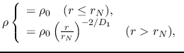 |
|
|
(4.97) |
as shown in Figure 4.12.
Since the free-fall-time of the gas contained in the inner core  is the same,
such gas reaches the center once.
It makes a very large accretion rate at
is the same,
such gas reaches the center once.
It makes a very large accretion rate at
 as
as
 .
If
.
If  ,
for
,
for
 .
Since
.
Since  and
and
 ,
equation (4.95) predicts
,
equation (4.95) predicts
 .
A constant accretion rate is expected for this power-law and
the accretion rate is converged to a constant value after
the stellar mass is much larger than than that was containd in
.
A constant accretion rate is expected for this power-law and
the accretion rate is converged to a constant value after
the stellar mass is much larger than than that was containd in  ,
,
 .
If
.
If  ,
,
 for
.
Since for this power
for
.
Since for this power  and
and
 ,
equation(4.95) predicts
,
equation(4.95) predicts
 .
They gave
.
They gave
 for
for  .
.
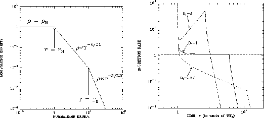
Figure 4.12:
A model proposed to explain time variation in accretion rate
by Henriksen, André, & Bontemps (1997).
The density distribution  at
at  (left) and expected accretion rate (right).
 |
Subsections
Kohji Tomisaka
2012-10-03