The ionization fraction of the gas in the cloud is low.
Neutral gas and the ions are coupled via mutual collisions and ions are coupled with the magnetic field.
Thus, the neutral molecules, a major component of the gas, are coupled with
the magnetic field indirectly via ionized ions.
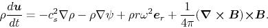
Equation of motion for the molecular gas is
 |
(4.47) |
where the forces appeared in the rhs represent, respectively,
the pressure force, the self-gravity, the centrifugal force, and the force exerted on
the neutral component per unit volume through two-body collision with ions.
The friction force has a form
 |
(4.48) |
We have assumed
 since the mass density of the charged component is
much smaller than that of the neutral one.
On the other hand, that for ions is
since the mass density of the charged component is
much smaller than that of the neutral one.
On the other hand, that for ions is
 |
(4.49) |
where we ignored the pressure and self-gravity forces compared with the Lorentz force.
If the inertia of the ions are ignored [lhs of eq.(4.49)=0],
equations (4.47) and (4.49) give the equation
of motion similar to that of the one-fluid as follows:
 |
(4.50) |
Ignoring the inertia of the ions, equation (4.49) indicates that
the friction force should be balanced with the Lorentz force as
 |
(4.51) |
Using equations (4.46) and (4.48),
this gives the drift velocity of ions against the neutrals as
Since the Lorentz force works outwardly, the drift velocity
 also points outwardly.
Viewing from the ions and magnetic field lines,
also points outwardly.
Viewing from the ions and magnetic field lines,
 points inwardly.
Thus, the mass in a flux tube varies with time;
that of the cloud center increases while that of the cloud surface decreases.
The ambipolar diffusion is a process to change the mass distribution against
the magnetic flux tube.
points inwardly.
Thus, the mass in a flux tube varies with time;
that of the cloud center increases while that of the cloud surface decreases.
The ambipolar diffusion is a process to change the mass distribution against
the magnetic flux tube.
It is useful to derive the timescale of ambipolar diffusion.
The characteristic timescale of magnetic flux loss is given
as
 , where
  represents the size of the cloud.
This gives
represents the size of the cloud.
This gives
This ambipolar diffusion timescale is several times longer than the
dynamical contraction timescale (eq.[2.26]) or
free-fall timescale as
Thus,
the magnetic flux of the cloud is not be lost
during the dynamical contraction ( free-fall).
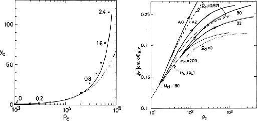
Figure 4.7:
Relation central density  against mass-to-flux ratio
  .
Plane-parallel and axisymmetric models are illustrated
in the left and right panels, respectively.
.
Plane-parallel and axisymmetric models are illustrated
in the left and right panels, respectively.
 |
How is the structure affected by the increase of mass/flux ratio at the cloud center?
Here, we will derive the relation between the mass-to-flux ratio and central density
and answer the question.
Numerical calculation is necessary for the axisymmetric (realistic) cloud.
However, this can be obtained for the case of a plane-parallel disk in which
the magnetic field is running parallel to the disk,
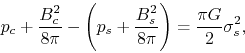
For the plane-parallel disk the hydrostatic balance is achieved as
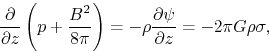 |
(4.57) |
where
 .
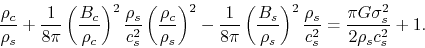
Equation (4.57) is integrated to obtain the
relation between the variables at the center
.
Equation (4.57) is integrated to obtain the
relation between the variables at the center  as
as
 |
(4.58) |
where we used
 .
This is rewritten as
.
This is rewritten as
 |
(4.59) |
In the second term of lhs,
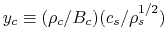 is a nondimensional mass flux ratio at the center and this is related to the
center-to-surface density ratio
is a nondimensional mass flux ratio at the center and this is related to the
center-to-surface density ratio
 .
Using these nondimensional variables, equation (4.59)
is expressed as
.
Using these nondimensional variables, equation (4.59)
is expressed as
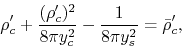 |
(4.60) |
where
 represents
the central density necessary for the disk to be supported without
a magnetic field (
represents
the central density necessary for the disk to be supported without
a magnetic field (
 ).
Figure 4.7 (left) illustrates this relation.
This shows that if the central mass-to-flux ratio increases (moving upward),
the central density increases.
In low density,
).
Figure 4.7 (left) illustrates this relation.
This shows that if the central mass-to-flux ratio increases (moving upward),
the central density increases.
In low density,
 ,
equation (4.60) indicates
that
,
equation (4.60) indicates
that
 .
This means that on the low density regime, the density increases but
the strength of magnetic field does not increase.
Equation (4.60) also indicates that
.
This means that on the low density regime, the density increases but
the strength of magnetic field does not increase.
Equation (4.60) also indicates that
 increase much as
 when
when
 .
This relation between mass-to-flux ratio and the central density is well
fitted to the numerical calculation of plane-parallel disk cloud driven by the ambipolar diffusion
by Mouschovias, Paleologou, & Fiedler (1985).
Does this indicate that the mass-to-flux ratio increases much when the central
density increases, for example, from
.
This relation between mass-to-flux ratio and the central density is well
fitted to the numerical calculation of plane-parallel disk cloud driven by the ambipolar diffusion
by Mouschovias, Paleologou, & Fiedler (1985).
Does this indicate that the mass-to-flux ratio increases much when the central
density increases, for example, from
 to
to
 ?
?
From this point, quasistatic evolution of the magnetized cloud was first studied
by Nakano (1979) adopting a method seeking for magnetohydrostatic configuration
(Mouschovias 1976a, 1976b).
He obtained that
the magnetic flux to mass ratio near the center of the cloud does not decrease much
below a critical density above which magnetohydrostatic configurations no more exist.
Paleologou & Mouschovias (1983), Shu (1983), and Mouschovias, Paleologou, & Fiedler (1985)
gave a completely different result.
That is, the magnetic flux to mass ratio near the center decreases much
when the density becomes larger than
 .
Critical discussion has been done between them4.1.
However, we have now realized that
the difference comes from the geometry assumed.
.
Critical discussion has been done between them4.1.
However, we have now realized that
the difference comes from the geometry assumed.
Relation of the mass-to-flux ratio to the central density for the axisymmetric realistic
(not plane-parallel disk) cloud is plotted in Figure 4.7 (right)
(Tomisaka, Ikeuchi, & Nakamura 1990).
The central mass-to-flux ratio increases by the ambipolar diffusion.
This increases the central density.
Lines with arrows indicate the evolutionary paths driven by the ambipolar diffusion.
It is to be noticed that
the relation is completely different from that of the plane-parallel disk.
Increase of the mass-flux ratio is small although the central density increases much.
This indicates that in the quasistatic evolution driven by the ambipolar diffusion
the mass-flux ratio does not increase much in contrast to the plane-parallel case.
In fully ionized plasma, the magnetic field is coupled to the matter.
However, in the low ionized gas the magnetic field is coupled only to the ions.
Thus the induction equation of magnatic field should be written
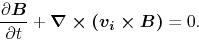 |
(4.61) |
This leads to the final expression as
![\begin{displaymath}
\frac{\partial \mbox{\boldmath${B}$}}{\partial t}+\mbox{\bol...
...ight)\mbox{\boldmath${\times B}$}\right]\times B\right\}}$}=0,
\end{displaymath}](img1185.png) |
(4.62) |
where we used the expression of the drift velocity [equation (4.52)].
In the isothermal cloud,
there is a maximum mass supported by the magnetic field.
Since in the subcritical cloud  the magnetic flux escapes from the center,
the critical mass decreases with time.
After the critical mass becomes smaller than the actual mass (
the magnetic flux escapes from the center,
the critical mass decreases with time.
After the critical mass becomes smaller than the actual mass (
 ),
there is no hydrostatic configuration.
The cloud evolves into the supercritical cloud region and experiences dynamical collapse.
),
there is no hydrostatic configuration.
The cloud evolves into the supercritical cloud region and experiences dynamical collapse.
Kohji Tomisaka
2009-12-10