Next: Mass Spectrum Up: Introduction Previous: T Tauri Disks Contents
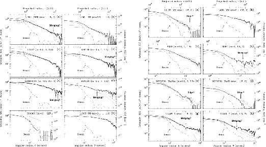
Motte & André (2001) made ![]() 1.3 mm continuum mapping survey of the embedded young stellar
objects (YSOs) in the Taurus molecular cloud.
Their maps include several isolated Bok globules, as well as protostellar objects in the Perseus cluster.
For the protostellar envelopes mapped in Taurus, the results are roughly consistent with the
predictions of the self-similar inside-out collapse model of Shu and collaborators (section 4.5.1).
The envelopes observed in Bok globules are also qualitatively consistent with these predictions,
providing the effects of magnetic pressure are included in the model.
By contrast, the envelopes of Class 0 protostars in Perseus have finite radii
1.3 mm continuum mapping survey of the embedded young stellar
objects (YSOs) in the Taurus molecular cloud.
Their maps include several isolated Bok globules, as well as protostellar objects in the Perseus cluster.
For the protostellar envelopes mapped in Taurus, the results are roughly consistent with the
predictions of the self-similar inside-out collapse model of Shu and collaborators (section 4.5.1).
The envelopes observed in Bok globules are also qualitatively consistent with these predictions,
providing the effects of magnetic pressure are included in the model.
By contrast, the envelopes of Class 0 protostars in Perseus have finite radii
![]() AU and are a factor of 3 to 12 denser than is predicted by the standard model.
AU and are a factor of 3 to 12 denser than is predicted by the standard model.
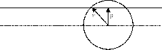
Another method to measure the density distribution is to use the near IR extinction.
From ![]() colors of background stars, the local value of
colors of background stars, the local value of ![]() in a dark cloud can
be obtained using a standard reddening law,
in a dark cloud can
be obtained using a standard reddening law,
| (1.13) |
See Figure 1.27.
If the density distribution is expressed as
| (1.15) |
| (1.16) |
| (1.17) |
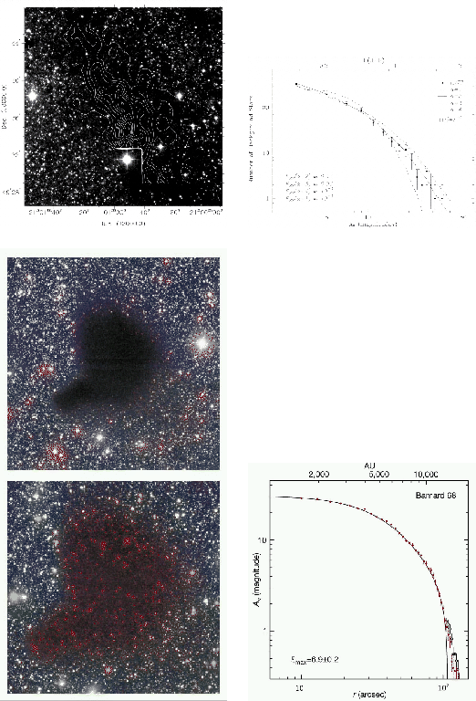
Recently, Alves et al (2001) derived directly the radial distribution of ![]() by comparing
the
by comparing
the ![]() model distribution for B68.
They obtained a distribution is well fitted by the Bonner-Ebert sphere in which
a hydrostatic balance between the self-gravity and the pressure force is achieved (lower panels
of Fig.1.29) (see section 4.1.1).
model distribution for B68.
They obtained a distribution is well fitted by the Bonner-Ebert sphere in which
a hydrostatic balance between the self-gravity and the pressure force is achieved (lower panels
of Fig.1.29) (see section 4.1.1).
 |
 |
In this fields, we should pay attention to the density distribution in cylindrical clouds.
As seen in the Taurus molecular cloud, there are many filamentary structures in a molecular cloud.
In ![]() 4.1, we will give
the distribution for a hydrostatic spherically symmetric and that of a cylindrical cloud.
The former is proportional to
4.1, we will give
the distribution for a hydrostatic spherically symmetric and that of a cylindrical cloud.
The former is proportional to
![]() and the latter is
and the latter is
![]() .
Therefore, the distribution
.
Therefore, the distribution
![]() was expected for cylindrical cloud.
From near IR extinctions observation (Alves et al 1998), even if a cloud is rather elongated
[Fig.1.29 (top-left)], the power of the density distribution is equal
to not
was expected for cylindrical cloud.
From near IR extinctions observation (Alves et al 1998), even if a cloud is rather elongated
[Fig.1.29 (top-left)], the power of the density distribution is equal
to not ![]() but
but ![]() .
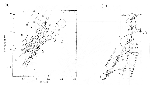
Fiege, & Pudritz (2001) proposed an idea that a toroidal component of the magnetic field,
.
Fiege, & Pudritz (2001) proposed an idea that a toroidal component of the magnetic field, ![]() ,
plays an important role in the hydrostatic balance of the cylindrical cloud (Fig.1.30).
,
plays an important role in the hydrostatic balance of the cylindrical cloud (Fig.1.30).
 |
Kohji Tomisaka 2012-10-03