Jeans Instability

Sound wave seems to be modified in the medium where the self-gravity is important. Beside the continuity equation (2.35)

$$\frac{\partial \delta \rho}{\partial t}+\rho_0 \frac{\partial \delta u}{\partial x}=0,$$ (2.45)

and the equation of motion (2.37)

$$\rho_0 \frac{\partial \delta u}{\partial t}= -c_{is}^2\frac... ...o}{\partial x}-\rho_0\frac{\partial \delta \phi}{\partial x},$$ (2.46)

the linearized Poisson equation

$$\frac{\partial^2 \delta \phi}{\partial x^2}=4\pi G \delta \rho,$$ (2.47)

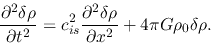
should be included. $\partial /\partial x\times$ (2.46) gives

$$\rho_0\left(\frac{\partial^2 \delta u}{\partial x \partial t... ...artial^2 \delta \rho}{\partial x^2}-4\pi G \rho_0 \delta \rho.$$ (2.48)

where we used equation (2.47) to eliminate $\delta \phi$. This yields

$$\frac{\partial^2 \delta \rho}{\partial t^2}=c_{is}^2 \frac{\partial^2 \delta \rho}{\partial x^2}+4\pi G \rho_0 \delta \rho.$$ (2.49)

where we used $\partial /\partial t\times$ (2.45).

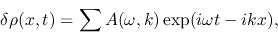
This is the equation which characterizes the growth of density perturbation owing to the self-gravity. Here we consider the perturbation are expressed by the linear combination of plane waves as

$$\delta \rho (x,t)=\sum A(\omega,k)\exp(i\omega t-ikx),$$ (2.50)

where $k$ and $\omega$ represent the wavenumber and the angular frequency of the wave. Picking up a plane wave and putting into equation (2.49), we obtain the dispersion relation for the gravitational instability as

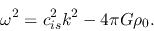$$\omega^2=c_{is}^2k^2 -4\pi G \rho_0.$$ (2.51)

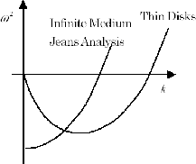
Reducing the density to zero, the equation gives us the same dispersion relation as that of the sound wave as $\omega /k=c_{is}$. For short waves ( $k \gg k_J=(4\pi G \rho_0)^{1/2}/c_{is}$), since $\omega^2>0$ the wave is ordinary oscillatory wave. Increasing the wavelength (decreasing the wavenumber), $\omega^2$ becomes negative for $k < k_J=(4\pi G \rho_0)^{1/2}/c_{is}$. For negative $\omega^2$, $\omega$ can be written $\omega =\pm i \alpha$ using a positive real $\alpha$. 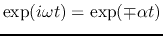In this case, since $\exp(i\omega t)=\exp(\mp \alpha t)$, the wave which has $\omega=-i\alpha$ increases its amplitude exponentially. This means that even if there are density inhomogeneities only with small amplitudes, they grow in a time scale of $1/\alpha$ and form density inhomogeneities with large amplitudes.

Figure 2.2: Dispersion Relation

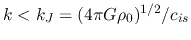
The critical wavenumber

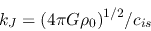$$k_J=(4\pi G \rho_0)^{1/2}/c_{is}$$ (2.52)

corresponds to the wavelength

$$\lambda_J=\frac{2\pi}{k_J}=\left(\frac{\pi c_{is}^2}{G \rho_0}\right)^{1/2},$$ (2.53)

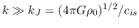
which is called the Jeans wavelength. Ignoring a numerical factor of the order of unity, it is shown that the Jeans wavelength is approximately equal to the free-fall time scale (eq.[2.26]) times the sound speed. The short wave with $\lambda \ll \lambda_J$ does not suffer from the self-gravity. For such a scale, the analysis we did in the preceding section is valid.

Typical values in molecular clouds, such as $c_{is}=200{\rm m s^{-1}}$, $\rho_0=2\times 10^{-20}{\rm g cm^{-3}}$, give us the Jeans wavelength as $\lambda_J=1.7\times 10^{18}{\rm cm}=0.56 {\rm pc}$. The mass contained in a sphere with a radius $r=\lambda_J/2$ is often called Jeans mass, which gives a typical mass scale above which the gas collapses. Typical value of the Jeans mass is as follows

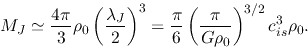$$M_J\simeq \frac{4\pi}{3}\rho_0\left(\frac{\lambda_J}{2}\righ... ...{\pi}{6}\left(\frac{\pi}{G \rho_0}\right)^{3/2}c_{is}^3\rho_0.$$ (2.54)

Using again the above typical values in the molecular clouds, $c_{is}=200{\rm m s^{-1}}$, $\rho_0=2\times 10^{-20}{\rm g cm^{-3}}$, the Jeans mass of this gas is equal to $M_J\simeq 27 M_\odot$.