Toomre's $Q$ Value

Consider the case of $m=0$ axisymmetric perturbations. Equation (3.32) becomes

$$\omega^2=k^2c_s^2 - 2\pi G \Sigma_0 \vert k\vert + \kappa^... ...\right)^2+\kappa^2-\left(\frac{\pi G \Sigma_0}{c_s}\right)^2.$$ (3.33)

If $\omega^2>0$ the system is stable against the axisymmetric perturbation, while if $\omega^2 < 0$ the system is unstable. Defining

$$Q=\frac{\kappa c_s}{\pi G \Sigma_0},$$ (3.34)

if $Q>1$, $\omega^2>0$ for all wavenumbers $k$. On the other hand, if $Q<1$, $\omega^2$ becomes negative for some wavenumbers $k_1 < k < k_2$. Therefore, the Toomre's $Q$ number gives us a criterion whether the system is unstable or not for the axisymmetric perturbation. [Recommendation for a reference book of this section: Binney & Tremaine (1988).]

The condition is expressed as

$$\Sigma_0 > \Sigma_{\rm cr}=\frac{\kappa c_s}{\pi G} (Q < 1).$$ (3.35)

Kennicutt plotted $\Sigma _0/\Sigma _{\rm cr}$ against the normalized radius as $R/R_{\rm HII}$ for various galaxies, where $R_{\rm HII}$ represents the maximum distance of HII regions from the center (Fig.3.8). Since $\Sigma_0/\Sigma_{\rm cr}=Q$, Figure 3.8 shows that HII regions are observed mainly in the region with $Q<1$ but those are seldom seen in the outer low-density $Q>1$ region. This seems the gravitational instability plays an important role.

Figure 3.8: $\Sigma_0/\Sigma_{\rm cr}$ vs $R/R_{\rm HII}$. $R_{\rm HII}$ represents the maximum distance of HII regions from the center. The sound speed is assumed constant $c_s=6{\rm km s}^{-1}$. Taken from Fig.11 of Kennicutt (1989).

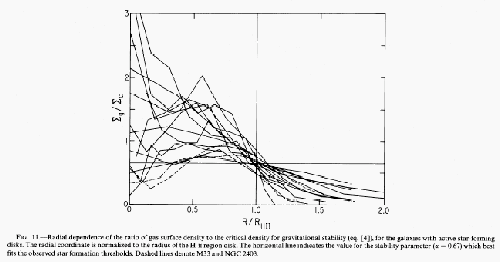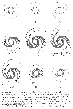
Figure: Numerical simulation of the swing amplification mechanism. The number attached each panel shows the time sequence. This is obtained by the time-dependent linear analysis. First, perturbation with leading spiral pattern is added to the Mestel disk with $Q=1.5$. The leading spiral gradually unwinds and become a trailing spiral. Loosely wound spiral pattern winds gradually and the last panel shows a tightly wound leading spiral pattern. The final amplitude is $\sim 100$ times larger than that of the initial state.

The above discussion is for the gaseous disk. The Toomre's $Q$ value is also defined for stellar system as

$$Q = \frac{\sigma_R \kappa}{3.36 G \Sigma_0},$$ (3.36)

where $\sigma_R$ represents the radial velocity dispersion.

For non-axisymmetric waves, even if $1\mbox{\raisebox{0.3ex}{$<$}\hspace{-1.1em} \raisebox{-0.7ex}{$\sim$}} Q \mbox{\raisebox{0.3ex}{$<$}\hspace{-1.1em} \raisebox{-0.7ex}{$\sim$}} 2$ the instability grows. To explain this, the swing amplification mechanism is proposed (Toomre 1981). If there is a leading spiral perturbation in the disk with $1\mbox{\raisebox{0.3ex}{$<$}\hspace{-1.1em} \raisebox{-0.7ex}{$\sim$}} Q \mbox{\raisebox{0.3ex}{$<$}\hspace{-1.1em} \raisebox{-0.7ex}{$\sim$}} 2$, the wave unwinds and finally becomes a trailing spiral pattern. At the same time, the amplitude of the wave (perturbations) is amplified (see Fig.3.9).