Observation of Mass-to-Flux Ratio

Figure 4.5 shows the mass-to-flux ratio normalized with the critical value

$$\lambda_C\equiv \frac{\left(\frac{M}{\Phi}\right)_{\rm obs}}{\left(\frac{M}{\Phi}\right)_{\rm crit}}$$ (4.43)

where

$$\left(\frac{M}{\Phi}\right)_{\rm crit}=\frac{1}{2\pi G^{1/2}}$$ (4.44)

is the critical mass-to-flux ratio which is obtained numerically from equation (4.31). $\lambda_C>1$ represents a supercritical cloud while $\lambda_C<1$ represents a subcritical cloud.

Figure 4.5: Mass-to-flux ratio is plotted against the column density. Dots are obtained from Zeeman splitting and stars are Chandrasekhar-Fermi method.

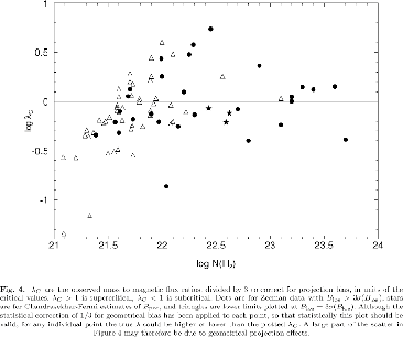Figure 4.5 indicates cloud cores are more or less found near the critical mass-to-flux ratio. They are not distributed either in the regions $\lambda_C \gg 1$ (very supercritical) or $\lambda_C \ll 1$ (very subcritical).