


Next: Basic Equations for Radiative
Up: Hydrostatic Equilibrium
Previous: Polytrope
Contents
In section 4.2, we obtained the maximum mass which is supported
against the self-gravity using the virial analysis.
In this section, we will survey result of more realistic calculation.
Formalism was obtained by Mouschovias (1976a,6), which was extended by
Tomisaka, Ikeuchi, & Nakamura (1988) to include the effect of rotation.
Magnetohydrostatic equlibrium is achived on a balance between the Lorentz
force, gravity, thermal pressure force, and the centrifugal force as
 |
(C.13) |
In the axisymmetric case, the poloidal magnetic fields is obtained by
the magnetic flux function,  ,
or the
,
or the  -component of the vector potential as
Equation (C.13) leads to
with
 |
(C.18) |
Equation (C.17) indicates  is a function of as
 , which is constant along one magnetic field line.
Ferraro's isorotation law demands,
that is, to satisfy the stead-state induction
equation
, which is constant along one magnetic field line.
Ferraro's isorotation law demands,
that is, to satisfy the stead-state induction
equation  is constant along a magnetic field.
This means is also constant along one magnetic field line,
is constant along a magnetic field.
This means is also constant along one magnetic field line,
 .
From this, the density distribution in one flux tube is written
.
From this, the density distribution in one flux tube is written
![\begin{displaymath}
\rho=\frac{q}{c_s^2}\exp\left[-\left(\psi-\frac{1}{2}r^2\omega^2\right)/c_s^2\right].
\end{displaymath}](img1524.png) |
(C.19) |
This means  is also constant along one magnetic field line,
  .
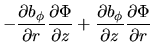
Since the forces are expressed by the defrivative of function
.
Since the forces are expressed by the defrivative of function
 |
(C.20) |
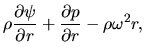
where equation (C.19) is used,
equation (C.15) and (C.16) are rewritten as
Finally, using the fact that  , , and are functions of ,
these two equations are reduced to
, , and are functions of ,
these two equations are reduced to
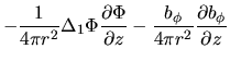
![\begin{displaymath}
\Delta_1 \Phi=-\frac{d (b_\phi^2/2)}{d \Phi}
-4\pi r^2 \lef...
.../c_s^2\right]+\rho r^2 \omega \frac{d \omega}{d \Phi}\right\}.
\end{displaymath}](img1533.png) |
(C.23) |
Another equation to be coupled is the Poisson equation as
![\begin{displaymath}
\Delta \psi=4\pi G \frac{q}{c_s^2}\exp\left[ -\left(\psi-\frac{1}{2}r^2\omega^2\right)/c_s^2\right].
\end{displaymath}](img1534.png) |
(C.24) |
The source terms of equations (C.23) and (C.24) are given by determining
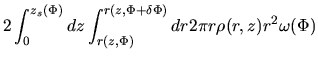
the mass
 and the angular momentum
 contained in a flux tube -
 .
Mass and angular momentum distribution of
.
Mass and angular momentum distribution of
is chosen artitrary in nature, where  is the the height of the cloud surface where
the magnetic potential is equal to .
For example,
is the the height of the cloud surface where
the magnetic potential is equal to .
For example,  and
and  are chosen
as a uniformly rorating uniform-density spherical cloud threaded by uniform magnetic field.
Since
are chosen
as a uniformly rorating uniform-density spherical cloud threaded by uniform magnetic field.
Since
The source terms of PDEs [eqs (C.23) and (C.24)] are given
from equations (C.27) and (C.28).
While the functons and are determined from the solution of these PDEs
after and are chosen.
This can be solved by a self-consistent field method.
Next: Basic Equations for Radiative
Up: Hydrostatic Equilibrium
Previous: Polytrope
Contents
Kohji Tomisaka
2007-07-08


![$\displaystyle -4\pi r^2\left\{\frac{\partial q}{\partial z}\exp\left[ -\left(\p...
...right)/c_s^2\right]+\rho r^2 \omega \frac{\partial \omega}{\partial z}\right\},$](img1529.png)
![$\displaystyle -4\pi r^2\left\{\frac{\partial q}{\partial r}\exp\left[ -\left(\p...
...right)/c_s^2\right]+\rho r^2 \omega \frac{\partial \omega}{\partial r}\right\}.$](img1531.png)


![$\displaystyle {\left(d m/d \Phi \right)}/{\int_0^{z_s(\Phi)} dz 2\pi \left(\par...
...ac{1}{c_s^2}\exp\left[ -\left(\psi-\frac{1}{2}r^2\omega^2\right)/c_s^2\right]},$](img1547.png)
![$\displaystyle {\left(d L/d \Phi \right)}/{\int_0^{z_s(\Phi)} dz 2\pi \left(\par...
...2}q(\Phi)r^2\exp\left[ -\left(\psi-\frac{1}{2}r^2\omega^2\right)/c_s^2\right]},$](img1549.png)