


Next: Tightly Wound Spirals
Up: Galactic Scale Star Formation
Previous: Local Star Formation Rate
Contents
Here, we will derive the dispersion relation for the gravitational instability of a rotating thin disk.
We will see the spatial variation of Toomre's  parameter, which determines the stability of the rotating disk,
explains the nonlinearity of star formation rate, that is, there is a threshold density and no stars are formed in the
low density region.
Use the cylindrical coordinate
parameter, which determines the stability of the rotating disk,
explains the nonlinearity of star formation rate, that is, there is a threshold density and no stars are formed in the
low density region.
Use the cylindrical coordinate  and the basic equations for thin disk in
  2.6.
In linear analysis, we assume
2.6.
In linear analysis, we assume
 ,
,
 ,
,
 ,
where
,
where  and
and  represent the radial and azimuthal components of the velocity.
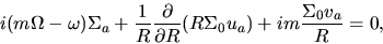
Linearized continuity equation is
represent the radial and azimuthal components of the velocity.
Linearized continuity equation is
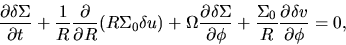 |
(3.8) |
where  .
Linearized equations of motion are
.
Linearized equations of motion are
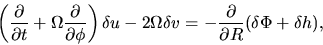 |
(3.9) |
and
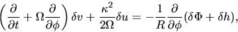 |
(3.10) |
where  is a specific enthalpy as
  and
and
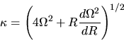 |
(3.11) |
is the epicyclic frequency.
We assume any solution of equations (3.8), (3.9) and(3.10) can be
written as a sum of terms of the form
![$\displaystyle \delta u = u_a \exp[i(m\phi-\omega t)],$](img703.png) |
|
|
(3.12) |
![$\displaystyle \delta v = v_a \exp[i(m\phi-\omega t)],$](img704.png) |
|
|
(3.13) |
![$\displaystyle \delta \Sigma = \Sigma_a \exp[i(m\phi-\omega t)],$](img705.png) |
|
|
(3.14) |
![$\displaystyle \delta h = h_a \exp[i(m\phi-\omega t)],$](img706.png) |
|
|
(3.15) |
![$\displaystyle \delta \Phi = \Phi_a \exp[i(m\phi-\omega t)].$](img707.png) |
|
|
(3.16) |
Using the equation of state of
 ,
,
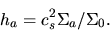 |
(3.17) |
Using equations (3.12)-(3.16),
equations (3.8), (3.9), and (3.10) are rewritten as
 |
(3.18) |
![\begin{displaymath}
u_a [\kappa^2 -(m\Omega -\omega)^2] = -i\left[ (m\Omega - \...
...\Phi_a + h_a) + 2m\Omega \frac{(\Phi_a + h_a)}{R} \right],
\end{displaymath}](img711.png) |
(3.19) |
and
![\begin{displaymath}
v_a [\kappa^2 -(m\Omega -\omega)^2] = \left[ \frac{\kappa^2...
..._a) + m (m\Omega-\omega) \frac{(\Phi_a + h_a)}{R} \right],
\end{displaymath}](img712.png) |
(3.20) |
Subsections
Next: Tightly Wound Spirals
Up: Galactic Scale Star Formation
Previous: Local Star Formation Rate
Contents
Kohji Tomisaka
2007-07-08