We have described the cloud run-away collapse and succeeding accretion process
In the latter phase, there is a possibility that the outflow is driven by the
effect of magnetic Lorentz force.
A restricted number of numerical simulation can simulate such evolution throughout.
The size of the molecular cores
![]() is more than
is more than ![]() times as large as
the typical size of the first core
times as large as
the typical size of the first core
![]() .
Therefore numerical scheme to calculate such process must have a large dynamic-range.
In the finite-difference scheme,
the spatial dynamic range is restricted by the number of the cells.
Although at least
.
Therefore numerical scheme to calculate such process must have a large dynamic-range.
In the finite-difference scheme,
the spatial dynamic range is restricted by the number of the cells.
Although at least
![]() grid points (in 2D) seems necessary
to resolve a factor of
grid points (in 2D) seems necessary
to resolve a factor of ![]() , to solve the MHD equation with the Poisson equation
of the self-gravity have not been done.
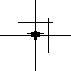
This is done by the Eularean nested-grid simulation.
This method uses a finite number of grid systems with different spatial resolutions are prepared.
Coarse grid covers whole the cloud and is to see a global structure.
Fine grid covers only the central part of the cloud and is to see the fine-scale structure
appeared near the center.
Figure 4.14 explains grid cells of the nested grid method.
The size of the cells of the
, to solve the MHD equation with the Poisson equation
of the self-gravity have not been done.
This is done by the Eularean nested-grid simulation.
This method uses a finite number of grid systems with different spatial resolutions are prepared.
Coarse grid covers whole the cloud and is to see a global structure.
Fine grid covers only the central part of the cloud and is to see the fine-scale structure
appeared near the center.
Figure 4.14 explains grid cells of the nested grid method.
The size of the cells of the ![]() -th level grid (L
-th level grid (L![]() ) is taken equal to
a half of those of the L
) is taken equal to
a half of those of the L![]() .
.
 |
A cylindrical cloud with coaxial magnetic field in hydrostatic balance is studied.
Rotation vector
![]() and the magnetic field
and the magnetic field
![]() are parallel to the symmetric
axis of the cylinder (
are parallel to the symmetric
axis of the cylinder (![]() -axis).
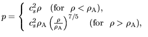
For the energy equation, a double-polytropic equation of state is adopted,
since the radiation hydrodynamical calculation (for example Masunaga & Inutsuka 2000)
predicts
-axis).
For the energy equation, a double-polytropic equation of state is adopted,
since the radiation hydrodynamical calculation (for example Masunaga & Inutsuka 2000)
predicts ![]() relations like shown in Figure 4.12,
which consists of a number of power-laws
for some density ranges.
relations like shown in Figure 4.12,
which consists of a number of power-laws
for some density ranges.
 |
(4.98) |
![\begin{displaymath}
\lambda_{\rm max} \simeq \frac{2\pi (1+\alpha/2+\beta)^{1/2}...
...ht)^{1/3}-0.6\right]^{1/2}}\frac{c_s}{(4 \pi G \rho_c)^{1/2}}.
\end{displaymath}](img1264.png) |
(4.99) |
![[*]](crossref.png) ) begins to be formed.
In the isothermal collapse phase,
a characteristic power-law for the Larson-Penston self-similar solution is seen
in the radial distributions of density as
) begins to be formed.
In the isothermal collapse phase,
a characteristic power-law for the Larson-Penston self-similar solution is seen
in the radial distributions of density as
After
![]() the first core is formed.
Radial infall motion is accelerated toward the surface of the first core and
the rotational motion
the first core is formed.
Radial infall motion is accelerated toward the surface of the first core and
the rotational motion ![]() also increases.
This amplification promotes the toroidal magnetic field,
also increases.
This amplification promotes the toroidal magnetic field, ![]() .
Since the torque is proportional to
.
Since the torque is proportional to
![]() ,
the amplitude of the torque increases after the first core formation.
,
the amplitude of the torque increases after the first core formation.
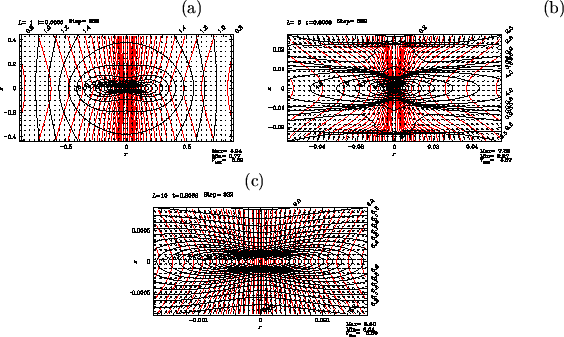
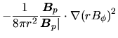
Structure just after ![]() 500 yr has passed from Figure 4.15 is shown
in Figure 4.15
In
500 yr has passed from Figure 4.15 is shown
in Figure 4.15
In ![]() yr from the epoch of Figure 4.15,
flow is completely changed and outflow is launched.
Panel (b), which corresponds to a four-times close-up of panel (a), shows clearly
that outflow is ejected from a region near
yr from the epoch of Figure 4.15,
flow is completely changed and outflow is launched.
Panel (b), which corresponds to a four-times close-up of panel (a), shows clearly
that outflow is ejected from a region near
![]() and
and
![]() .
And the outflow vectors and the disk has an gngle of approximately 45 deg.
The magneto-centrifugal wind model favors a small angle between the magnetic field and the disk,
.
And the outflow vectors and the disk has an gngle of approximately 45 deg.
The magneto-centrifugal wind model favors a small angle between the magnetic field and the disk,
![]() deg.
This model predicts that the angle between the flow and the disk is also smaller than 60 deg.
Numerical results is not inconsistent with this prediction of magneto-centrifugal wind model.
deg.
This model predicts that the angle between the flow and the disk is also smaller than 60 deg.
Numerical results is not inconsistent with this prediction of magneto-centrifugal wind model.
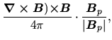
To see which force is driving such outflow, amplitudes of three forces are compared:
the Lorentz force
![]() ,
the centrifugal force
,
the centrifugal force
![]() ,
and the thermal pressure gradient
,
and the thermal pressure gradient
![]() .
The parallel components to the poloidal magnetic field of the three forces are as
.
The parallel components to the poloidal magnetic field of the three forces are as
 |
 |
||
 |
(4.100) |
| (4.101) |
| (4.102) |
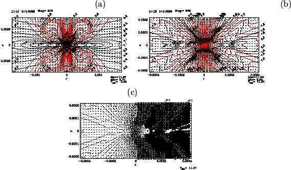
Difference between models with different magnetic field strength but the same rotation speed is
illustrated in Figure 4.17.
Magnetic to thermal pressure ratio ![]() is taken 1 [panels (a), and (d)],
0.1 [panels (b), and (e)], and 0.01 [panels (c), and (f)].
Panels (a), (b), (c) in the left column are snapshots when the central density reaches
is taken 1 [panels (a), and (d)],
0.1 [panels (b), and (e)], and 0.01 [panels (c), and (f)].
Panels (a), (b), (c) in the left column are snapshots when the central density reaches ![]() while
panels (d), (e), (f) in the right column show the structure after
while
panels (d), (e), (f) in the right column show the structure after
![]() passed.
In the model with
passed.
In the model with ![]() , the outflow gas flows through a region whose shape resembles a capital letter U.
This is similar to that observed in model (
, the outflow gas flows through a region whose shape resembles a capital letter U.
This is similar to that observed in model (![]() and
and ![]() )
shown in Figure 4.16.
Decreasing the magnetic field strength
)
shown in Figure 4.16.
Decreasing the magnetic field strength
![]() and
and
![]() ,
the shape of disk changes from a flat disk to a round ellipsoid.
The model with neither magnetic field nor rotation shows a spherical contracting core.
Outflow is also affected by decrease in magnetic field strength.
Globally folded magnetic field lines are seen in the outflow region in panel (e).
Smaller-scale structure folding the magnetic field lines develops in the outflow region in panel (f).
The strucure seen in the polidal magnetic field is well correlated to the distribution of toroidal magnetic field
strength.
That is, a packet of strong
,
the shape of disk changes from a flat disk to a round ellipsoid.
The model with neither magnetic field nor rotation shows a spherical contracting core.
Outflow is also affected by decrease in magnetic field strength.
Globally folded magnetic field lines are seen in the outflow region in panel (e).
Smaller-scale structure folding the magnetic field lines develops in the outflow region in panel (f).
The strucure seen in the polidal magnetic field is well correlated to the distribution of toroidal magnetic field
strength.
That is, a packet of strong ![]() pinch the gas and poloidal magnetic field lines radially inwardly.
This means that the toroidal magnetic field is amplified by the rotation motion and becomes predominant over
the poloidal one in the case with meak initial magnetic field.
Thus, the whoop stress, which is expressed by the first term of the Lorentz force of equation(B.13)
and comes from the tension of toroidal magnetic field, pinches the plasma contained inside of the loop of
pinch the gas and poloidal magnetic field lines radially inwardly.
This means that the toroidal magnetic field is amplified by the rotation motion and becomes predominant over
the poloidal one in the case with meak initial magnetic field.
Thus, the whoop stress, which is expressed by the first term of the Lorentz force of equation(B.13)
and comes from the tension of toroidal magnetic field, pinches the plasma contained inside of the loop of
![]() .
For this case, the magnetic force dominant region is widely spread compared with the centrifugal force
dominant region, which is far from the model with strong magnetic field.
In this case, the magnetic pressure gradient plays an important role.
Gas of outflow is ejected perpendicularly from the disk and forms flow similar to the capital letter I.
In conclusion,
U-type and I-type outflows are generated for strong magnetic model and weak magnetic model, respectively.
.
For this case, the magnetic force dominant region is widely spread compared with the centrifugal force
dominant region, which is far from the model with strong magnetic field.
In this case, the magnetic pressure gradient plays an important role.
Gas of outflow is ejected perpendicularly from the disk and forms flow similar to the capital letter I.
In conclusion,
U-type and I-type outflows are generated for strong magnetic model and weak magnetic model, respectively.
 |
 |